Module 4: Entropy and Uncertainty¶

The problem with only looking at the top score¶

In Module 3, we left our Monday ticket here:

account_unlock:    0.576
vpn_issue:         0.386
security_incident: 0.039

Margin = 0.19 — too close to auto-route. We sent it to clarification queue.

Now consider a different ticket that just came in — an outage report:

account_unlock:    0.58
vpn_issue:         0.21
security_incident: 0.21

The top score is almost identical (0.58 vs 0.576). The margin is different (0.37 vs 0.19). By the routing rules from Module 3, the outage report actually looks safer — higher margin.

But look more carefully. In the outage report, two classes are tied at 0.21. The model isn't just uncertain between first and second — it's equally lost between second and third. The uncertainty is spreading, not concentrating.

Your margin metric can't see this. You need a new tool: entropy.

What entropy measures¶

Entropy is a single number that captures how spread out a probability distribution is.

\[ H(P) = -\sum_{i=1}^{n} P(i) \log_2 P(i) \]

Two anchor points to memorise:

Entropy = 0 → all probability sits on one class. The model is certain.

[1.00, 0.00, 0.00]   →   H = 0

Entropy = log₂(n) → probability is split perfectly evenly. The model is maximally lost.

[0.33, 0.33, 0.33]   →   H = log₂(3) = 1.585 bits

Everything else falls between those two poles.

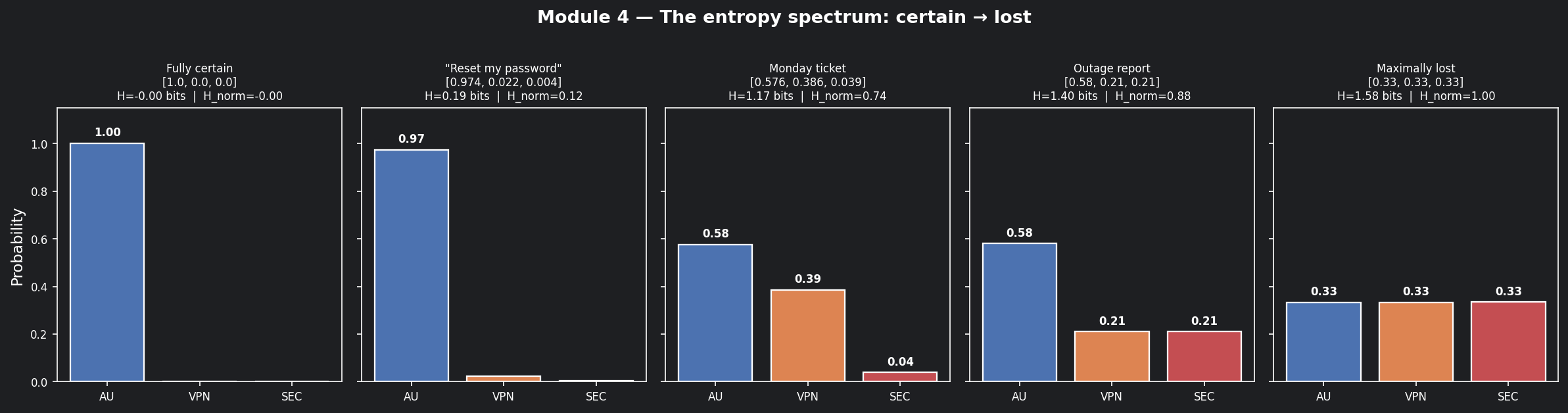
📊 Visualisation 1 — The entropy spectrum: from certain to lost¶

This chart shows five distributions along the spectrum from H=0 to H=1.585, so you can see what "certain", "uncertain", and "maximally lost" actually look like as bar charts before we apply entropy to our tickets.

Let's calculate it on the Monday ticket¶

Ticket 1 — Monday's ambiguous ticket:

P = [0.576, 0.386, 0.039]

H = -(0.576 × log₂0.576) + (0.386 × log₂0.386) + (0.039 × log₂0.039)
  = -(0.576 × -0.796)    + (0.386 × -1.374)    + (0.039 × -4.678)
  =   0.458              +   0.530              +   0.182
  = 1.17 bits

Ticket 2 — The outage report:

P = [0.58, 0.21, 0.21]

H = -(0.58 × log₂0.58) + (0.21 × log₂0.21) + (0.21 × log₂0.21)
  = -(0.58 × -0.786)   + (0.21 × -2.252)   + (0.21 × -2.252)
  =   0.456             +   0.473            +   0.473
  = 1.40 bits

Maximum possible entropy for 3 classes = log₂(3) = 1.585 bits.

Ticket	Top score	Margin	Entropy	Assessment
Monday ticket	0.576	0.190	1.17 bits	Uncertain — clarification queue
Outage report	0.580	0.370	1.40 bits	More uncertain — escalate faster

The top scores are nearly identical. The outage report has a higher margin. But entropy reveals it is closer to maximum confusion — something margin completely missed.

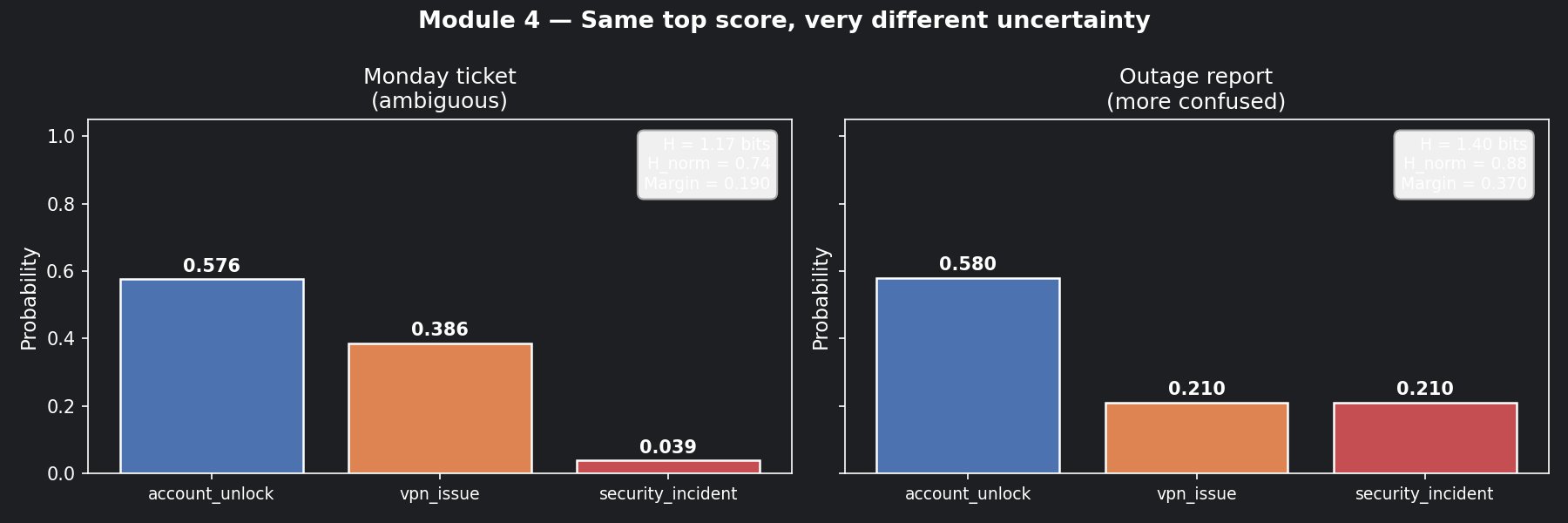
📊 Visualisation 2 — Monday ticket vs outage report: side by side¶

This chart puts the two tickets next to each other with their entropy scores, making it obvious why margin alone is not enough.

Normalised entropy: comparing across different class counts¶

Raw entropy values only make sense within the same number of classes. A 3-class problem maxes at 1.585 bits; a 10-class problem maxes at 3.32 bits. You can't compare them directly.

Normalise to a 0–1 scale:

\[ H_{norm} = \frac{H(P)}{\log_2 n} \]

Now 0 always means "fully certain" and 1 always means "fully lost" — regardless of how many classes your classifier uses.

Ticket	Raw entropy	Normalised entropy
"Reset my password" (Module 3)	~0.15 / 1.585	~0.09
Monday ticket	1.17 / 1.585	0.74
Outage report	1.40 / 1.585	0.88

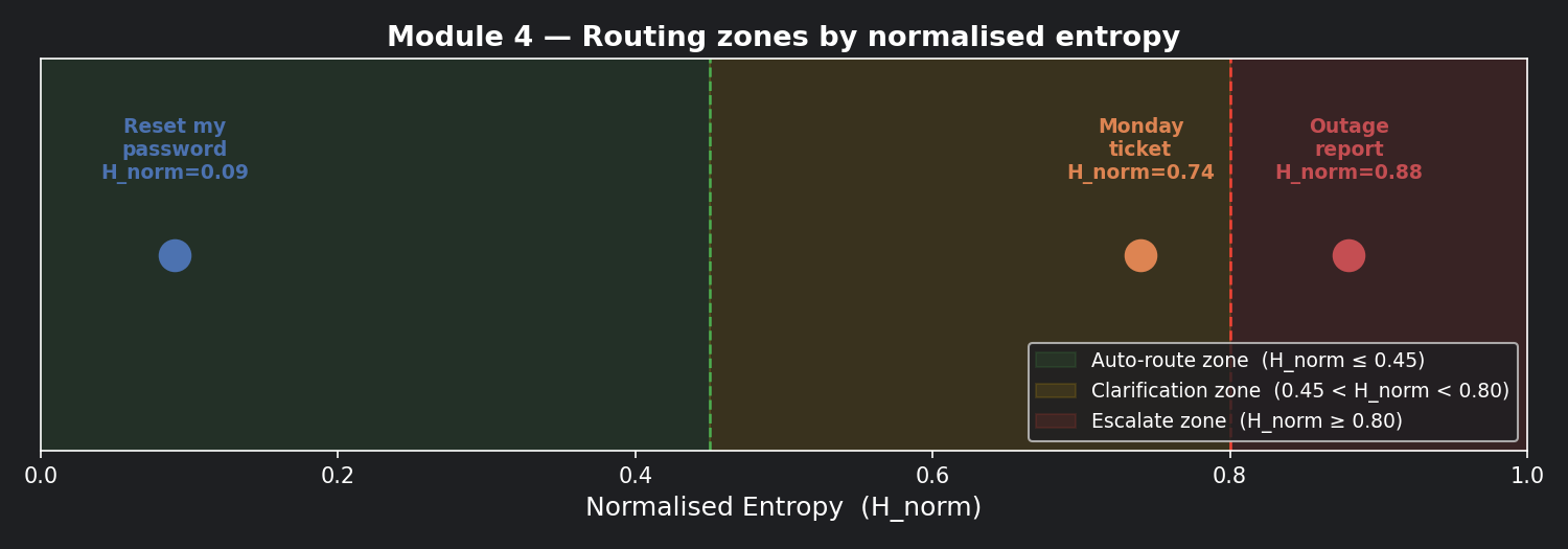
📊 Visualisation 3 — Normalised entropy on a 0–1 scale with routing zones¶

This is the chart to bookmark. It maps H_norm onto a colour-coded axis with your three routing zones marked — so you can see at a glance where each ticket lands relative to the decision boundaries.

The combined routing policy¶

Each metric from Modules 2–4 catches a different failure mode:

Failure mode	What it looks like	Which metric catches it
Model is unsure between top two	Top score 0.60, second 0.55	Margin (Module 3)
Model spreads uncertainty widely	Top 0.58, others all similar	Entropy (this module)
Model looks confident but is often wrong	Top score 0.80, historically 40% wrong	Calibration (Module 8)

A robust routing policy uses all three:

if top_prob >= 0.80 and margin >= 0.60 and H_norm <= 0.45:
    route_to_specialist()          # all three gates pass
elif H_norm >= 0.80:
    escalate_immediately()         # too confused to act safely
else:
    send_to_clarification_queue()  # something didn't clear

Applied to our three tickets:

Ticket	Top prob	Margin	H_norm	Decision
"Reset my password"	0.974	0.952	0.09	✅ Auto-route
Monday ticket	0.576	0.190	0.74	🔁 Clarification queue
Outage report	0.580	0.370	0.88	🚨 Escalate immediately

Three different outcomes from three superficially similar top scores.

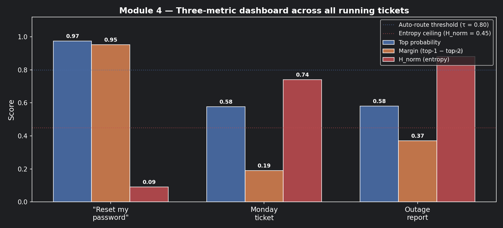
📊 Visualisation 4 — All three tickets: the three-metric dashboard¶

This chart shows all three metrics side by side for all three tickets — the most useful view for understanding why each routing decision is different.

Why this matters for security incidents specifically¶

Misrouting a security incident to a tier-1 agent doesn't just waste time — it leaves an active threat unaddressed.

Entropy is your last line of defence before auto-routing on ambiguous tickets. A ticket with H_norm = 0.88 should never be auto-routed, regardless of what the top class says. The model is telling you it genuinely doesn't know. Listen to it.

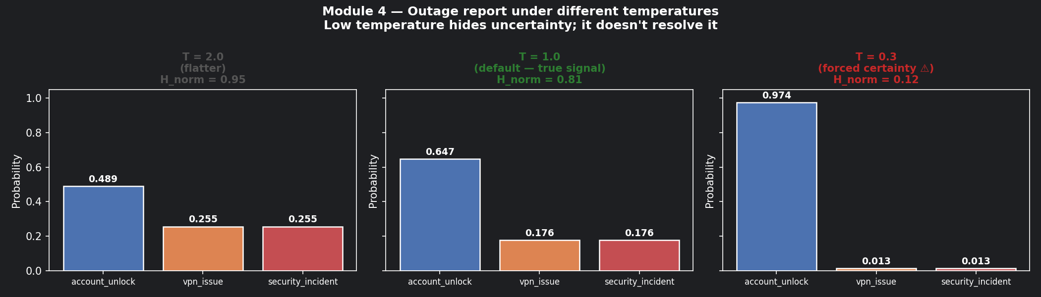
The instinct to override high entropy with a low temperature setting (from Module 3) is exactly the wrong move here. Sharpening a confused distribution doesn't resolve the confusion — it just makes it invisible until something breaks in production.

📊 Visualisation 5 — What low temperature does to a high-entropy distribution¶

This shows why using T=0.3 to "fix" the outage report is dangerous. The distribution looks confident. The underlying uncertainty hasn't changed.

How to practice this¶

Open notebooks/math-foundations/04_entropy.ipynb and work through:

Run Visualisation 1 — place a new ticket distribution on the spectrum and read its H_norm
Calculate raw and normalised entropy for all three running-scenario tickets by hand, then verify with code
Build the combined routing policy (top prob + margin + entropy) and test it on a sample queue
Run Visualisation 5 — confirm that T=0.3 on the outage report would push it past the auto-route threshold. Would you trust that decision?

Checklist before moving on¶

[ ] Can you explain why two tickets with the same top score can have very different entropy?
[ ] Are you calculating normalised entropy so it's comparable across different classifier sizes?
[ ] Does your routing policy combine top probability, margin, and entropy — not just one?
[ ] Do high-entropy tickets (H_norm ≥ 0.80) have an explicit fast-escalation path?
[ ] Has someone tuned your entropy threshold against real historical outcomes, not just held-out test data?

Where Module 5 picks up¶

We now have a routing policy that works correctly on individual tickets. But the question Module 5 asks is different:

"Run this policy on 30 days of tickets. Does it behave the same way every day — or does quality swing wildly depending on what comes in?"

The tool for answering that is variance and standard deviation.