Distance Metrics: Measuring Similarity

There are multiple ways to measure "similarity" between two embedding vectors. Each has trade-offs. This section covers the math and practical implications.

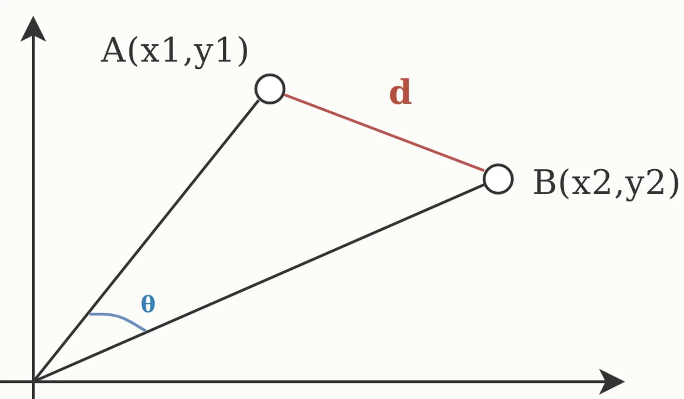
Cosine Similarity (Most Common)

Definition

Given normalized vectors $\hat{\vec{u}}$ and $\hat{\vec{v}}$ (each with magnitude 1):

\[\text{cosine\_similarity}(\vec{u}, \vec{v}) = \hat{\vec{u}} \cdot \hat{\vec{v}} = \frac{\vec{u} \cdot \vec{v}}{\|\vec{u}\| \cdot \|\vec{v}\|}\]

This equals the cosine of the angle between vectors:

\[\cos(\theta) = \frac{\vec{u} \cdot \vec{v}}{\|\vec{u}\| \cdot \|\vec{v}\|}\]

Properties

Range: $[-1, 1]$
1: identical direction (most similar)
0: perpendicular (completely different)
-1: opposite direction (least similar)

Why It's Used in RAG

Normalized embeddings: Most models output unit-length vectors
Angle-based: Captures "direction" not "magnitude"
Fast: Just a dot product after normalization
Invariant to scale: Longer passage ≈ shorter passage if similar content

Example

import numpy as np

# Two passages about cats
vec_passage1 = np.array([0.1, 0.9, 0.2, 0.0])  # (normalized)
vec_passage2 = np.array([0.15, 0.85, 0.25, 0.05])  # (similar, normalized)
vec_passage3 = np.array([0.8, 0.1, 0.05, 0.3])  # (about dogs, normalized)

# Cosine similarity
sim_1_2 = np.dot(vec_passage1, vec_passage2)
sim_1_3 = np.dot(vec_passage1, vec_passage3)

print(f"Cat-Cat similarity: {sim_1_2:.3f}")  # ≈ 0.975
print(f"Cat-Dog similarity: {sim_1_3:.3f}")  # ≈ 0.256

When to Use

✅ Use cosine similarity when: - Vectors are normalized (most embedding models do this) - Document length varies widely - You care about content direction, not magnitude

❌ Avoid when: - Vectors have important magnitude information - Document length is meaningful signal

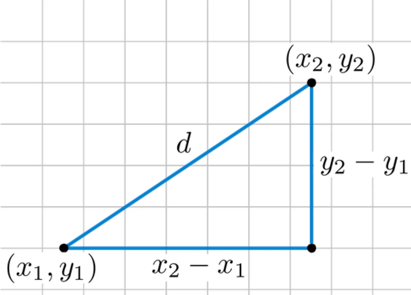
Euclidean Distance

Definition

For vectors $\vec{u}$ and $\vec{v}$:

\[d_{\text{Euclidean}}(\vec{u}, \vec{v}) = \sqrt{\sum_{i=1}^{n} (u_i - v_i)^2} = \|\vec{u} - \vec{v}\|\]

This is the straight-line distance in space.

Properties

Range: $[0, \infty)$
0: identical vectors
Larger values: more different
Sensitive to magnitude: longer documents have larger distances

Relationship to Cosine

For normalized vectors, there's a mathematical relationship:

\[d_{\text{Euclidean}}^2 \approx 2(1 - \cos(\theta))\]

So Euclidean distance and cosine similarity give similar ranking for normalized vectors, but Euclidean is slower to compute.

Example

import numpy as np

u = np.array([1, 2, 3])
v = np.array([4, 5, 6])

# Manual
euclidean = np.sqrt((4-1)**2 + (5-2)**2 + (6-3)**2)
print(f"Euclidean distance: {euclidean:.3f}")  # 5.196

# Using numpy
euclidean = np.linalg.norm(u - v)
print(f"Using numpy: {euclidean:.3f}")  # 5.196

# Using scipy
from scipy.spatial.distance import euclidean as scipy_euclidean
print(f"Using scipy: {scipy_euclidean(u, v):.3f}")  # 5.196

When to Use

✅ Use Euclidean distance when: - Vectors are not normalized - Vector magnitude is meaningful - You're in low dimensions

❌ Avoid in RAG because: - Embedding models output normalized vectors - Slower than cosine similarity - Less semantically meaningful for text

Dot Product (Inner Product)

Definition

Simply the dot product without normalization:

\[d_{\text{dot}}(\vec{u}, \vec{v}) = \vec{u} \cdot \vec{v} = \sum_{i=1}^{n} u_i v_i\]

Properties

Range: $(-\infty, \infty)$
Larger values: more similar
Sensitive to magnitude: longer vectors = larger products
Fast: single multiplication and sum

Comparison to Cosine

For normalized vectors ($\|\vec{u}\| = \|\vec{v}\| = 1$):

\[d_{\text{dot}} = \text{cosine\_similarity}\]

But for unnormalized vectors, dot product depends on both direction AND magnitude.

Example

# Unnormalized vectors
u = np.array([2, 3, 4])
v = np.array([1, 2, 3])

# Dot product
dot = np.dot(u, v)
print(f"Dot product: {dot}")  # 2*1 + 3*2 + 4*3 = 2 + 6 + 12 = 20

# If we scale u, dot product changes even though direction is same
u_scaled = u * 2
dot_scaled = np.dot(u_scaled, v)
print(f"Dot product (u scaled): {dot_scaled}")  # 40

# But cosine similarity stays the same
cos_sim_1 = np.dot(u, v) / (np.linalg.norm(u) * np.linalg.norm(v))
cos_sim_2 = np.dot(u_scaled, v) / (np.linalg.norm(u_scaled) * np.linalg.norm(v))
print(f"Cosine similarities: {cos_sim_1:.3f}, {cos_sim_2:.3f}")  # Same!

When to Use

✅ Use dot product when: - Vectors are normalized (same as cosine then) - You need maximum speed - Magnitude information is important

❌ Avoid when: - Vectors have varying magnitudes - You need scale-invariant comparison

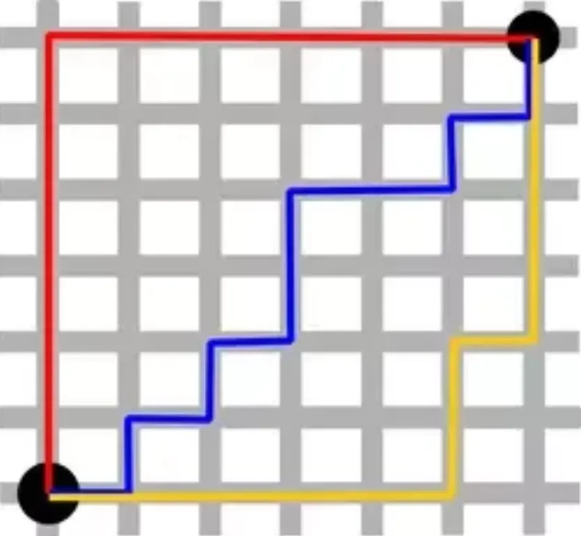
Manhattan Distance (L1)

Definition

\[d_{\text{Manhattan}}(\vec{u}, \vec{v}) = \sum_{i=1}^{n} |u_i - v_i|\]

Like the distance traveled on a city grid (you can only move horizontally/vertically).

When to Use

Rarely in RAG, but sometimes useful for: - Sparse vectors (mostly zeros) - Special structured data - More robust to outliers than Euclidean

from scipy.spatial.distance import cityblock

u = np.array([1, 2, 3])
v = np.array([4, 5, 6])

manhattan = cityblock(u, v)
print(f"Manhattan distance: {manhattan}")  # |4-1| + |5-2| + |6-3| = 3+3+3 = 9

Comparison Table

Metric	Formula	Range	Type	RAG Use	Speed
Cosine	$\frac{\vec{u} \cdot \vec{v}}{\\|\vec{u}\\|\\|\vec{v}\\|}$	[-1, 1]	Angle	✅ Best	Fast
Euclidean	$\sqrt{\sum(u_i-v_i)^2}$	[0, ∞)	Distance	⚠ Avoid	Slow
Dot	$\sum u_i v_i$	(-∞, ∞)	Similarity	✅ Good	Fast
Manhattan	$\sum \\|u_i-v_i\\|$	[0, ∞)	Distance	❌ Rare	Medium

Which Metric to Choose?

Decision Tree:

Are your vectors normalized to unit length?
├─ YES → Use cosine similarity or dot product
│        ├─ Need maximum speed? → Dot product
│        └─ Standard choice → Cosine similarity
│
└─ NO → Use Euclidean distance
        (but consider normalizing first)

For RAG systems: - 99% of the time: Cosine Similarity - Some vector DB defaults: Dot Product (equivalent for normalized) - Rarely: Euclidean or Manhattan

Maximum Inner Product Search (MIPS)

When using dot product, the problem becomes: find vectors with maximum dot product (not minimum distance).

This is called MIPS (Maximum Inner Product Search).

If you normalize vectors to unit length: $$\text{argmax}_i (\vec{q} \cdot \vec{v}_i) = \text{argmax}_i \cos(\theta_i)$$

So MIPS on normalized vectors = nearest neighbor in cosine similarity.

Code Example with Different Metrics

from sentence_transformers import SentenceTransformer
import numpy as np
from sklearn.metrics.pairwise import cosine_similarity

model = SentenceTransformer('all-MiniLM-L6-v2')

# Create some embeddings
docs = [
    "Cats are cute and furry",
    "Dogs are loyal pets",
    "Cats like to sleep and play",
    "Python is a programming language"
]

embeddings = model.encode(docs)

# Query
query = "I like my cat"
query_emb = model.encode([query])[0]

# Different metrics
cosine_sims = cosine_similarity([query_emb], embeddings)[0]
dot_products = np.dot(embeddings, query_emb)
euclidean_dists = np.linalg.norm(embeddings - query_emb, axis=1)

# Rank by each metric
cosine_rank = np.argsort(-cosine_sims)[:3]
dot_rank = np.argsort(-dot_products)[:3]
euclidean_rank = np.argsort(euclidean_dists)[:3]

print("Top 3 by cosine:", [docs[i] for i in cosine_rank])
print("Top 3 by dot:", [docs[i] for i in dot_rank])
print("Top 3 by euclidean:", [docs[i] for i in euclidean_rank])

# For normalized embeddings, cosine and dot give same ranking
print("Cosine and dot rankings same?", np.array_equal(cosine_rank, dot_rank))

Summary

Concept	Use In RAG
Cosine similarity	✅ Best choice for RAG
Dot product	✅ Good if normalized
Euclidean	⚠ Avoid (slower, less meaningful)
Manhattan	❌ Rarely useful

Next Steps

→ Exact vs Approximate Search - How to search millions of vectors fast

→ Vector Databases - Production systems

Metric	Formula	Range	Type	RAG Use	Speed
Cosine	\(\frac{\vec{u} \cdot \vec{v}}{\\|\vec{u}\\|\\|\vec{v}\\|}\)	[-1, 1]	Angle	✅ Best	Fast
Euclidean	\(\sqrt{\sum(u_i-v_i)^2}\)	[0, ∞)	Distance	⚠ Avoid	Slow
Dot	\(\sum u_i v_i\)	(-∞, ∞)	Similarity	✅ Good	Fast
Manhattan	\(\sum \\|u_i-v_i\\|\)	[0, ∞)	Distance	❌ Rare	Medium