Experiment 2: Top-p (Nucleus Sampling)¶

Who it's for: Anyone who completed Experiment 1 and wants to understand nucleus sampling deeply.
What you'll get: The ability to look at any top-p graph and immediately understand what it's telling you — and why top-p behaves so differently from temperature.

Before You Start: The Problem Temperature Alone Doesn't Solve¶

You learned in Experiment 1 that temperature reshapes probability distributions. But temperature has a fundamental limitation: it always includes every token in the sampling pool.

Even at T=0.5, tokens with logit=-1.0 still have some probability. Usually tiny — but "tiny" adds up when you're generating thousands of tokens. Occasionally the model will sample from these near-zero tokens, producing surprising or incoherent output.

Top-p(Nucleus Sampling) solves this by asking a different question:

Instead of "how do I reshape the probabilities?", it asks:
"Which tokens together account for most of the probability mass — and can I just ignore the rest?"

This is a fundamentally different kind of intervention.

Top-p in one line

Top-p is a candidate-set filter, not a global reshaping control.

The Core Intuition: The Probability Budget¶

Think of probability as a budget of 1.0 (or 100%).

At baseline (T=1.0), our 10 tokens spend that budget like this:

approve    → 0.36  (36%)
reject     → 0.24  (24%)
review     → 0.16  (16%)
escalate   → 0.10  (10%)
delay      → 0.05  (5%)
audit      → 0.04  (4%)
optimize   → 0.03  (3%)
notify     → 0.02  (2%)
assign     → 0.01  (1%)
close      → 0.01  (<1%)
Total:        1.00  (100%)

Top-p says: "I only want to spend my probability budget on the most important tokens."

p = 0.5 means: "Find the fewest tokens that together use up 50% of the budget — ignore the rest."
p = 0.9 means: "Find the fewest tokens that together use up 90% of the budget — ignore the rest."
p = 1.0 means: "Include everything — no filtering at all."

The set of tokens you keep is called the nucleus.

Memory hook

p is your probability budget; the nucleus is the smallest set that spends that budget.

Step 1: Understand the Algorithm — Exactly How Top-p Works¶

Here is the top-p algorithm, step by step:

Start with the probability distribution after softmax (optionally after temperature scaling)
Sort all tokens from highest to lowest probability
Walk down the sorted list, accumulating probability Stop when the cumulative sum first reaches or exceeds p
The tokens you've accumulated = the nucleus
Discard all other tokens (set their probability to zero)
Renormalize: divide each surviving token's probability by the total nucleus probability (so they sum to 1.0 again)
Sample from this renormalized nucleus

The key word is "smallest set". Top-p finds the minimum number of tokens needed to cover probability p. No more, no less.

Operational consequence

Two prompts with the same p can produce very different nucleus sizes.

Step 2: Trace the Algorithm Manually¶

Let's run through top-p = 0.8 by hand, using our token list.

Starting distribution (T=1.0, already sorted):

Rank  Token      Probability   Cumulative
  1   approve    0.360         0.360
  2   reject     0.240         0.600
  3   review     0.160         0.760
  4   escalate   0.100         0.860   ← first point where cumulative ≥ 0.80
  5   delay      0.050         0.910
  6   audit      0.040         0.950
  7   optimize   0.030         0.980
  8   notify     0.020         1.000
  9   assign     0.010         1.010
 10   close      0.010         1.020

With p = 0.80:

Walk down the list until cumulative sum ≥ 0.80:

After approve: 0.36 → not yet
After reject: 0.60 → not yet
After review: 0.76 → not yet
After escalate: 0.86 → crossed 0.80, stop here

Nucleus = {approve, reject, review, escalate}

Discard: delay, audit, optimize, notify, assign, close (set to 0)

Renormalize the nucleus:

Total nucleus probability = 0.360 + 0.240 + 0.160 + 0.100 = 0.860

approve   → 0.360 / 0.860 = 0.419  (41.9%)
reject    → 0.240 / 0.860 = 0.279  (27.9%)
review    → 0.160 / 0.860 = 0.186  (18.6%)
escalate  → 0.100 / 0.860 = 0.116  (11.6%)
Total:                      1.000  (100%)

Now sample from just these four tokens.

Notice what changed: approve went from 36% → 41.9%. All the discarded tokens' probability got redistributed to the survivors. The ranking stays the same, but the numbers shift upward slightly.

Step 3: Trace Three More p Values¶

Let's see how the nucleus changes across the five experiment runs:

p = 0.20¶

Walk down until cumulative ≥ 0.20: - After approve: 0.36 → already crossed 0.20, stop

Nucleus = {approve} — only ONE token!

Renormalized: approve = 100%

This is essentially deterministic. No matter how many times you sample, you always get approve.

p = 0.50¶

Walk down until cumulative ≥ 0.50: - After approve: 0.36 → not yet - After reject: 0.60 → crossed 0.50, stop

Nucleus = {approve, reject}

Renormalized:

approve → 0.360 / 0.600 = 60.0%
reject  → 0.240 / 0.600 = 40.0%

Only two choices. Every sample is either approve (60%) or reject (40%).

p = 0.95¶

Walk down until cumulative ≥ 0.95: - approve: 0.36 - reject: 0.60 - review: 0.76 - escalate: 0.86 - delay: 0.91 - audit: 0.95 → crossed 0.95, stop

Nucleus = {approve, reject, review, escalate, delay, audit} — 6 tokens

Renormalized: all 6 tokens divided by 0.95 ≈ each goes up slightly.

p = 1.00¶

Walk down until cumulative ≥ 1.00: This requires all 10 tokens.

Nucleus = everything. No filtering occurs. Equivalent to not using top-p at all.

Summary Table¶

p = 0.20  →  1 token  in nucleus  (approve only)
p = 0.50  →  2 tokens in nucleus  (approve, reject)
p = 0.80  →  4 tokens in nucleus  (approve, reject, review, escalate)
p = 0.95  →  6 tokens in nucleus  (approve through audit)
p = 1.00  → 10 tokens in nucleus  (everything)

The pattern: as p increases, more tokens enter the nucleus. The nucleus grows to match the probability you're willing to "spend."

What to internalize

p controls coverage, not a fixed number of candidates.

Step 4: The Dynamic Property — Why This Matters More Than You Think¶

Here is the most important concept in Experiment 2, and the reason top-p is preferred over top-k in most production systems.

The nucleus size changes depending on how confident the model is.

To see this, compare the same p=0.90 applied to two different distributions:

Distribution A: Model is very confident (peaked)¶

Token A1   0.82
Token A2   0.10
Token A3   0.05
Token A4   0.02
Token A5   0.01

Walk with p=0.90: - A1: 0.82 — not yet - A2: 0.92 — crossed! Stop.

Nucleus = {A1, A2} — just 2 tokens. The model is so sure that 90% of the budget is spent in 2 tokens.

Distribution B: Model is very uncertain (flat)¶

Token B1   0.15
Token B2   0.13
Token B3   0.12
Token B4   0.11
Token B5   0.10
Token B6   0.10
Token B7   0.09
Token B8   0.08
Token B9   0.07
Token B10  0.05

Walk with p=0.90: - B1: 0.15 - B2: 0.28 - B3: 0.40 - B4: 0.51 - B5: 0.61 - B6: 0.71 - B7: 0.80 - B8: 0.88 - B9: 0.95 — crossed! Stop.

Nucleus = {B1 through B9} — 9 tokens. The model is so unsure that even 9 tokens only cover 95% of the budget.

Same p=0.90. One case: 2 tokens. Other case: 9 tokens.

This is why it's called "dynamic" nucleus sampling. The nucleus size adapts to the shape of the distribution automatically. No tuning needed.

Common mistake

Assuming p=0.9 means the same number of tokens every time leads to incorrect tuning decisions.

Step 5: Temperature vs Top-p — The Exact Difference¶

This is the comparison that confuses most people. Both affect which token gets sampled — but they work at completely different stages and in completely different ways.

Temperature: changes the shape of the whole distribution¶

Before temperature:   [0.36, 0.24, 0.16, 0.10, 0.05, 0.04, 0.03, 0.02, 0.01, 0.01]
After T=0.5:          [0.61, 0.27, 0.09, 0.02, 0.00, 0.00, 0.00, 0.00, 0.00, 0.00]
After T=2.0:          [0.20, 0.17, 0.14, 0.11, 0.09, 0.08, 0.08, 0.07, 0.06, 0.05]

Every token is still there. Every token still has some probability. The shape changed, but nobody was excluded.

Top-p: cuts off the tail entirely¶

Before top-p:         [0.36, 0.24, 0.16, 0.10, 0.05, 0.04, 0.03, 0.02, 0.01, 0.01]
After p=0.80:         [0.42, 0.28, 0.19, 0.12,  0,    0,    0,    0,    0,    0  ]
After p=0.50:         [0.60, 0.40,  0,    0,    0,    0,    0,    0,    0,    0  ]

The tail is gone. Zeroed out. Those tokens can never be sampled, no matter what.

The operational difference¶

Question	Temperature	Top-p
Can the 10th-ranked token ever be sampled?	Yes, always	Only if p=1.0
Does the ranking of surviving tokens change?	Yes (e^x math can shift ranks at extreme T)	No, never
Does it help with very long generation loops?	Somewhat	Yes, strongly
What does "more" do?	More temperature = more random across all tokens	More top-p = more tokens eligible

When to use which¶

Situation	Use Temperature	Use Top-p
Want more variety in phrasing	✓
Want to completely block low-quality tokens		✓
Generating long sequences where tail tokens cause loops		✓
Want smooth gradation from focused to random	✓
Want a hard cutoff with no bleed-through		✓

In practice: Most systems use both. Temperature first (to reshape), then top-p (to trim the tail).

Division of labor

Temperature decides distribution shape; top-p decides who remains eligible.

Step 6: Read the Graphs — Panel by Panel¶

The graph exp2_top_p.png has 8 panels across 3 rows. Here is how to read each one.

Graph reading strategy

Start with dynamic nucleus size (row 2 left), then verify with cumulative curves (row 2 right).

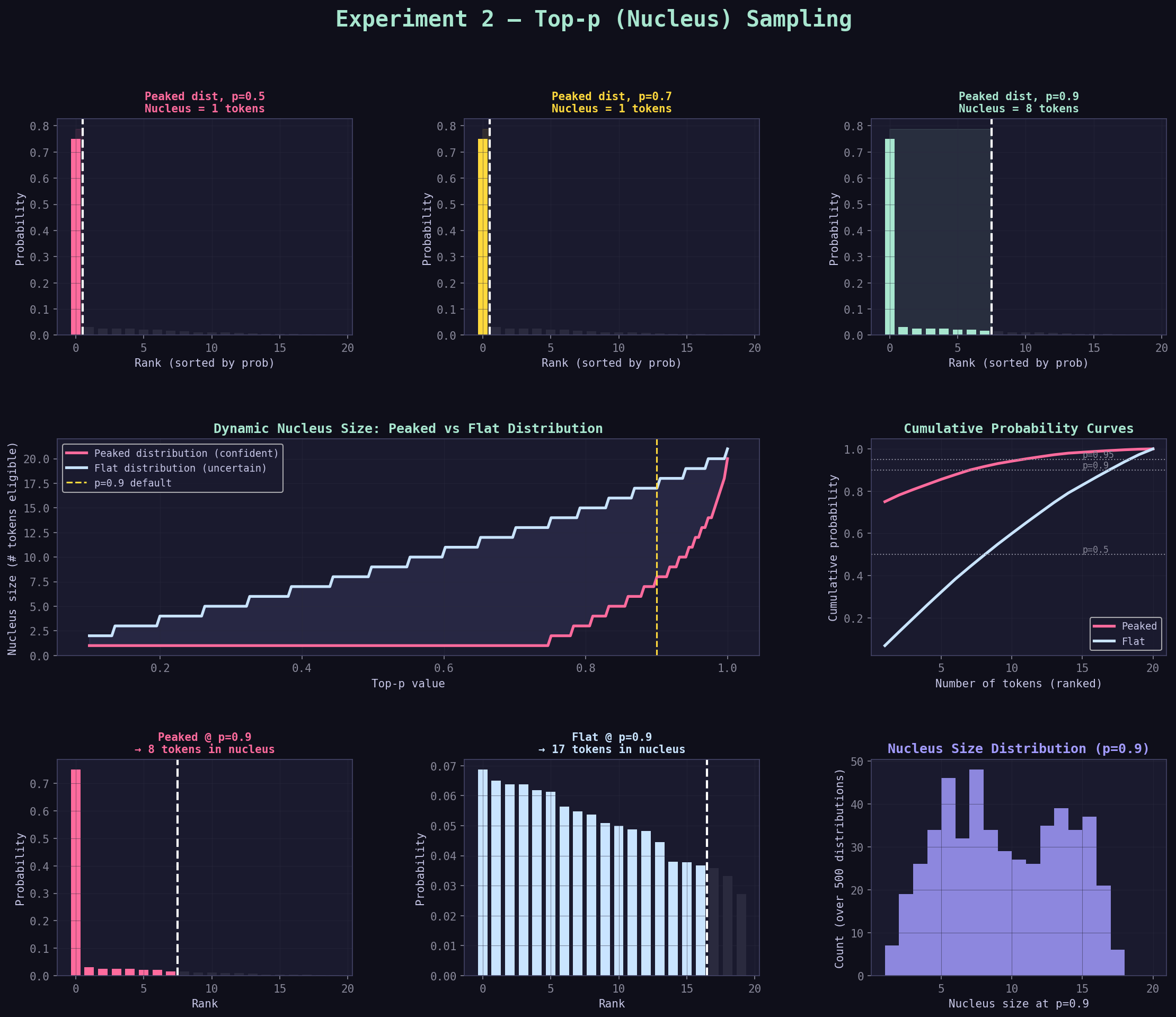
Row 1, Panels 1–3: "Peaked dist, p=X — Nucleus = N tokens"¶

These three bar charts show the nucleus for three different p values applied to the peaked distribution.

What you're looking at:

X-axis: tokens sorted from highest to lowest probability (rank order, not token index)
Y-axis: probability
Colored bars: tokens inside the nucleus
Dark (near-black) bars: tokens outside the nucleus (discarded)
White dashed vertical line: the nucleus cutoff boundary
Colored shaded region: the nucleus area

How to read it:

p=0.50 panel:  2 colored bars, 18 dark bars
               → Nucleus has only 2 tokens
               → The vertical line is very far left
               → The shaded region is tiny

p=0.70 panel:  More colored bars, fewer dark bars
               → Nucleus grew to include more tokens
               → The vertical line moved right

p=0.90 panel:  Even more colored bars
               → Nucleus grew again
               → The cutoff is now much further right

What the relative bar heights tell you:

After top-p is applied, the surviving bars don't change in relative order — but they shift upward slightly because the normalization step redistributes the discarded tokens' probability to the survivors. The taller bars grow taller, the shorter bars grow a bit too. This is the renormalization effect.

Row 2, Left: "Dynamic Nucleus Size: Peaked vs Flat Distribution"¶

This is the most important graph in the panel. It directly visualizes the dynamic property.

What you're looking at: - X-axis: p value (from 0.1 to 1.0) - Y-axis: number of tokens in the nucleus - Pink line: nucleus size for the peaked distribution - Blue line: nucleus size for the flat distribution - Yellow dashed line: p=0.9 (the common default) - Shaded area between lines: the "gap" showing how differently they behave

How to read it:

The pink line (peaked distribution) stays very low for most of the range. It doesn't need many tokens to cover p=0.9 because a few tokens already dominate.

The blue line (flat distribution) rises steeply. It needs many more tokens to reach the same p because the probability is spread evenly.

The key observation: At p=0.9 (yellow line), read across to where each line hits it. The pink line hits it at maybe 2–3 tokens. The blue line hits it at 12–15 tokens. Same p value, wildly different nucleus size.

The shaded gap between lines: This is your visual intuition for "how dynamic is top-p?" The bigger the gap, the more top-p is adapting to the distribution. A large gap is a good thing — it means top-p is doing its job of adjusting to context.

What the slope of each line means:

A steep slope means nucleus size grows quickly as p increases — many tokens are "roughly equally" probable, so each increment of p adds several tokens. A flat slope means nucleus size grows slowly — a few tokens dominate, so p can grow a lot before needing to add another token.

Row 2, Right: "Cumulative Probability Curves"¶

This graph shows the raw data that the top-p algorithm is walking through.

What you're looking at:

X-axis: number of tokens accumulated (rank 1, 2, 3, ...)
Y-axis: cumulative probability
Pink line: cumulative sum for the peaked distribution
Blue line: cumulative sum for the flat distribution
Three dotted horizontal lines: p=0.5, p=0.9, p=0.95

How to read it:

Each line starts at the bottom-left and rises to 1.0 at the top-right.

The pink line rises steeply at first — one token covers most of the probability — then flattens out. This is the visual signature of a peaked distribution.

The blue line rises gradually and nearly linearly — no single token dominates. This is the visual signature of a flat distribution.

Reading nucleus size from this graph:

Draw a horizontal line at your target p (e.g., 0.9). Where it crosses each curve, drop a vertical line to the x-axis. That x-value is your nucleus size.

For the peaked distribution at p=0.9: the horizontal line crosses the pink curve at about x=3. Nucleus = 3 tokens.

For the flat distribution at p=0.9: the horizontal line crosses the blue curve at about x=13. Nucleus = 13 tokens.

Pro tip: The shape of these curves tells you everything about how top-p will behave on a given distribution. A curve that jumps steeply = small nucleus. A curve that rises slowly = large nucleus.

Fast diagnostic

Steep cumulative curve means confident model output; shallow curve means uncertainty.

Row 3, Panels 1–2: "Peaked @ p=0.9" and "Flat @ p=0.9"¶

These two panels show the practical impact of the dynamic property side by side.

Left panel (Peaked @ p=0.9):

You'll see most bars are dark — a small nucleus. The cutoff line appears early in the rank order.

Right panel (Flat @ p=0.9):

You'll see most bars are colored — a large nucleus. The cutoff line appears late in the rank order.

The visual "aha" moment: Same p=0.9 setting. Completely different behavior. This is the whole point of top-p — it adapts.

Row 3, Right: "Nucleus Size Distribution (p=0.9)"¶

This histogram shows what happens when you apply p=0.9 to 500 randomly generated distributions.

What you're looking at:

X-axis: nucleus size (how many tokens were included)
Y-axis: how many of the 500 distributions produced that nucleus size

How to read it:

The histogram shows the range of possible nucleus sizes you encounter "in the wild." It's rarely a fixed number. Most distributions produce a nucleus of somewhere between 2 and 10 tokens at p=0.9, with a peak somewhere in between.

Why this matters:

If you were using top-k instead of top-p, you'd have to pick one fixed k value. But as this histogram shows, the "right" k would vary from 1 to 15+ depending on the distribution. Top-p handles all of these automatically with a single p=0.9 setting.

Step 7: The Renormalization Effect — Often Overlooked¶

When top-p cuts tokens from the tail, it doesn't just remove them. It renormalizes the remaining probabilities so they still sum to 1.0.

This has a subtle but important effect:

Before filtering (p=0.5 example):

approve  0.360  (36%)
reject   0.240  (24%)  ← cumulative = 60%, past p=0.5, so we stop here
[rest discarded]

The nucleus has total probability = 0.360 + 0.240 = 0.600 (60%)

After renormalization:

approve  0.360 / 0.600 = 0.600  (60%)   ← was 36%, now 60%
reject   0.240 / 0.600 = 0.400  (40%)   ← was 24%, now 40%

What changed:

The ratio between approve and reject stayed the same (3:2 → still 3:2). But both probabilities increased because the "discarded" 40% got folded back in.

The practical consequence:

When you apply p=0.5, you're not just "removing" the bottom 50% of tokens. You're implicitly saying: "Pretend the model only knows these top tokens. Renormalize as if they're the whole universe."

This is why very low p values make output feel more confident than even a low temperature would — not only are bottom tokens removed, but the top tokens each get a boosted probability.

Renormalization trap

Post-filter probabilities are sampling weights after exclusion, not raw model confidence.

Step 8: The Sample Output — How to Read It¶

From the original experiment, the output at p=0.20 looks like:

=== Top-p=0.2 (very tight) ===
Entropy: 0.721
approve       0.667
reject        0.333
review        0.000
escalate      0.000
delay         0.000
audit         0.000
optimize      0.000
notify        0.000
assign        0.000
close         0.000

Reading guide:

What you see	What it means
`Entropy: 0.721`	Low but not zero — two tokens survive, so there's some randomness
`approve 0.667`	66.7% chance — higher than the raw 36% because of renormalization
`reject 0.333`	33.3% chance — higher than the raw 24% for same reason
All others `0.000`	Completely excluded. These cannot be sampled.

Notice that approve went from 36% (baseline) to 66.7% (p=0.20). That's the renormalization at work — cutting reject from the pool would push approve to 100%, but since reject survives the p=0.20 threshold, the remaining 33.3% stays with reject.

Now the p=0.80 output:

=== Top-p=0.8 (loose) ===
Entropy: 2.234
approve       0.240
reject        0.198
review        0.167
escalate      0.116
delay         0.058
audit         0.047
optimize      0.000
notify        0.000
assign        0.000
close         0.000

Reading guide:

What you see	What it means
`Entropy: 2.234`	Higher — 6 tokens survive, more randomness
`approve 0.240`	24.0% — lower than its baseline 36%
All six survive	Renormalization spread probability across 6 tokens
Last four `0.000`	Still excluded, even though p=0.80 is fairly high

Wait — approve went from 36% → 24%? Yes. When the nucleus gets larger, the renormalization effect works in reverse — the probability gets spread more thinly. The top token's share decreases even though it's still the most likely choice.

Key insight from the output tables: Watching how approve's probability changes across p values teaches you the renormalization dynamic. It rises when p is very tight (fewer tokens, each gets more), falls when p is looser (more tokens, probability shared), and equals the original (36%) when p=1.0 (no filtering, no renormalization needed).

Step 9: Temperature + Top-p Together — How They Interact¶

From the optional dive deeper section:

# T=0.5, p=0.5
# T=1.0, p=0.5
# T=1.5, p=0.5

What does this show? Temperature changes the shape of the distribution that top-p then cuts.

Case 1: T=0.5, then p=0.5

At T=0.5, the distribution is already peaked. approve might have 0.61 probability. The cumulative sum crosses 0.50 after just the first token. Nucleus = {approve} only.

Effect: p=0.5 does almost nothing extra. Temperature already did the focusing.

Case 2: T=1.0, then p=0.5

Baseline distribution. cumulative crosses 0.50 after approve (0.36) and reject (0.24). Nucleus = {approve, reject}.

Case 3: T=1.5, then p=0.5

At T=1.5, the distribution is flatter. approve might have 0.28 probability. cumulative crosses 0.50 after approve + reject + review. Nucleus = 3 tokens.

The pattern:

Low temperature → distribution already peaked → top-p has less work to do → small nucleus
High temperature → distribution flatter → top-p has more to cut → larger nucleus
Same p, but nucleus size varies wildly depending on temperature.

This is why order matters in the pipeline:

Raw Logits → Temperature (reshape) → Top-p (trim) → Sample

Temperature decides how many tokens deserve inclusion; top-p enforces the actual cutoff. If you run top-p before temperature, you'd get completely different (and usually wrong) behavior.

Ordering matters

Applying top-p on the wrong distribution stage can invalidate your intended control behavior.

Step 10: Common Misconceptions — Cleared Up¶

Misconception 1: "p=0.9 means the model uses 90% of its vocabulary"

No. p=0.9 means the model keeps the fewest tokens whose probabilities sum to 0.9. In a peaked distribution, that might be 2 tokens. In a flat distribution, that might be 20 tokens. The percentage refers to cumulative probability, not vocabulary fraction.

Misconception 2: "Lower p is always safer"

Lower p focuses the model on fewer tokens — which can be good for accuracy. But too low a p (like p=0.2) can cause the model to repeat itself, because the same 1–2 tokens keep winning. It also kills any chance of creative or varied output. "Safe" depends entirely on your task.

Misconception 3: "Top-p and temperature do the same thing"

They're complementary, not equivalent. Temperature reshapes the whole distribution — every token's probability changes. Top-p then applies a hard cut, removing tokens entirely. You can have high temperature + low top-p (many tokens get probability, but only the top few are actually used) or low temperature + high top-p (distribution already focused, top-p barely does anything). They interact but they're not redundant.

Misconception 4: "The probability assigned to a token after top-p is its 'real' probability"

No. The probability after renormalization is an artifact of which other tokens survived. If review is in a nucleus with 4 tokens, it gets a different probability than if it's in a nucleus with 8 tokens. The renormalized probabilities are sampling weights, not the model's actual confidence in each token.

Misconception 5: "I should always use top-p"

Top-p can cause problems with very uniform distributions — it may include almost all tokens even at p=0.9. Some practitioners use top-k as a "safety ceiling" alongside top-p (see Experiment 4). For most tasks, top-p alone with p=0.9 is an excellent default.

Healthy default

Start with p=0.9, then move down for precision tasks or up for exploratory tasks.

Step 11: Practical Decision Guide¶

Use this when choosing your top-p setting:

Does your task have one correct answer?
    YES → p = 0.5 to 0.7  (tight nucleus, focus on top tokens)
    NO  → Is quality still important (not just exploration)?
              YES → p = 0.8 to 0.92  (standard production range)
              NO  → p = 0.95 to 1.0  (let the model breathe)

Real-World Settings¶

Calibration tip

Keep task metric fixed and sweep only p first before touching other parameters.

Task	Recommended p	Why
Classification	0.5	Usually top 1–2 tokens are the answer
Factual QA	0.7	Small nucleus, correct answer usually dominant
Code generation	0.85–0.95	Needs focus but some token variety for style
Summarization	0.9	Quality matters but phrasing can vary
Creative writing	0.95	Allow unusual word choices
Brainstorming	1.0	No filtering — let the model explore
Long generation	0.9	Helps prevent repetition loops

Step 12: What to Do Next¶

Top-p is the most commonly used sampling filter. Now you can go deeper:

Experiment 3 (Top-k): Top-k is a simpler version — instead of a probability threshold, it just keeps the k highest-probability tokens. It's less adaptive than top-p but easier to reason about. You'll see exactly where it falls short.
Experiment 4 (Combined): How do temperature, top-p, and top-k interact when used together? This is where you learn the full production pipeline.

Quick Reference: Graph Interpretation Cheat Sheet¶

When you open exp2_top_p.png, scan in this order:

1. Look at the nucleus cutoff panels (row 1)
   → Where is the dashed vertical line?
   → Far left = tight nucleus (low p)
   → Far right = large nucleus (high p)
   → How many bars are colored vs dark?

2. Look at the dynamic nucleus chart (row 2, left)
   → How far apart are the peaked vs flat lines?
   → Big gap = top-p is very adaptive to distribution shape
   → At p=0.9 (yellow line), read the nucleus size for each distribution

3. Look at the cumulative curves (row 2, right)
   → Does the curve rise steeply (peaked) or gradually (flat)?
   → Steep = small nucleus at any p value
   → Draw mental horizontal lines at 0.5, 0.9, 0.95 to read nucleus sizes

4. Look at the side-by-side comparison (row 3, left two panels)
   → Visually confirm the dynamic property:
     same p=0.9, different nucleus sizes

5. Look at the histogram (row 3, right)
   → What's the range of nucleus sizes?
   → This is how variable the behavior would be if you used top-k with a fixed number

Summary¶

Concept	One-sentence explanation
Top-p	Keep the smallest set of tokens whose probabilities sum to at least p
Nucleus	The tokens that survive the top-p filter
Dynamic	The nucleus size adapts automatically to how peaked or flat the distribution is
Renormalization	After filtering, surviving tokens' probabilities are rescaled to sum to 1.0
p=1.0	No filtering — identical to not using top-p at all
p=0.9	Standard default: keeps 90% of probability mass, cuts the tail
Temperature first	Temperature reshapes logits; top-p then trims the result

Final takeaway: Top-p is a "quality filter" that removes the model's worst ideas before sampling. The magic is that it automatically tightens when the model is confident and loosens when the model is unsure — adapting to context without you having to change anything.

Bottom line

Top-p is adaptive by construction; use that adaptivity intentionally.